LLMs and the Transformer Architecture, End to End
Co-authored by Claude Opus 4.8
This blog is summarized via my personal notes on the Transformer architecture, which is the backbone of Large Language Models (LLMs) like Claude and GPT. It provides a detailed walkthrough of the entire process, from tokenization to generating a probability distribution over the vocabulary, highlighting key components such as Q/K/V computation, attention mechanisms, and the differences between encoder-decoder and decoder-only models.
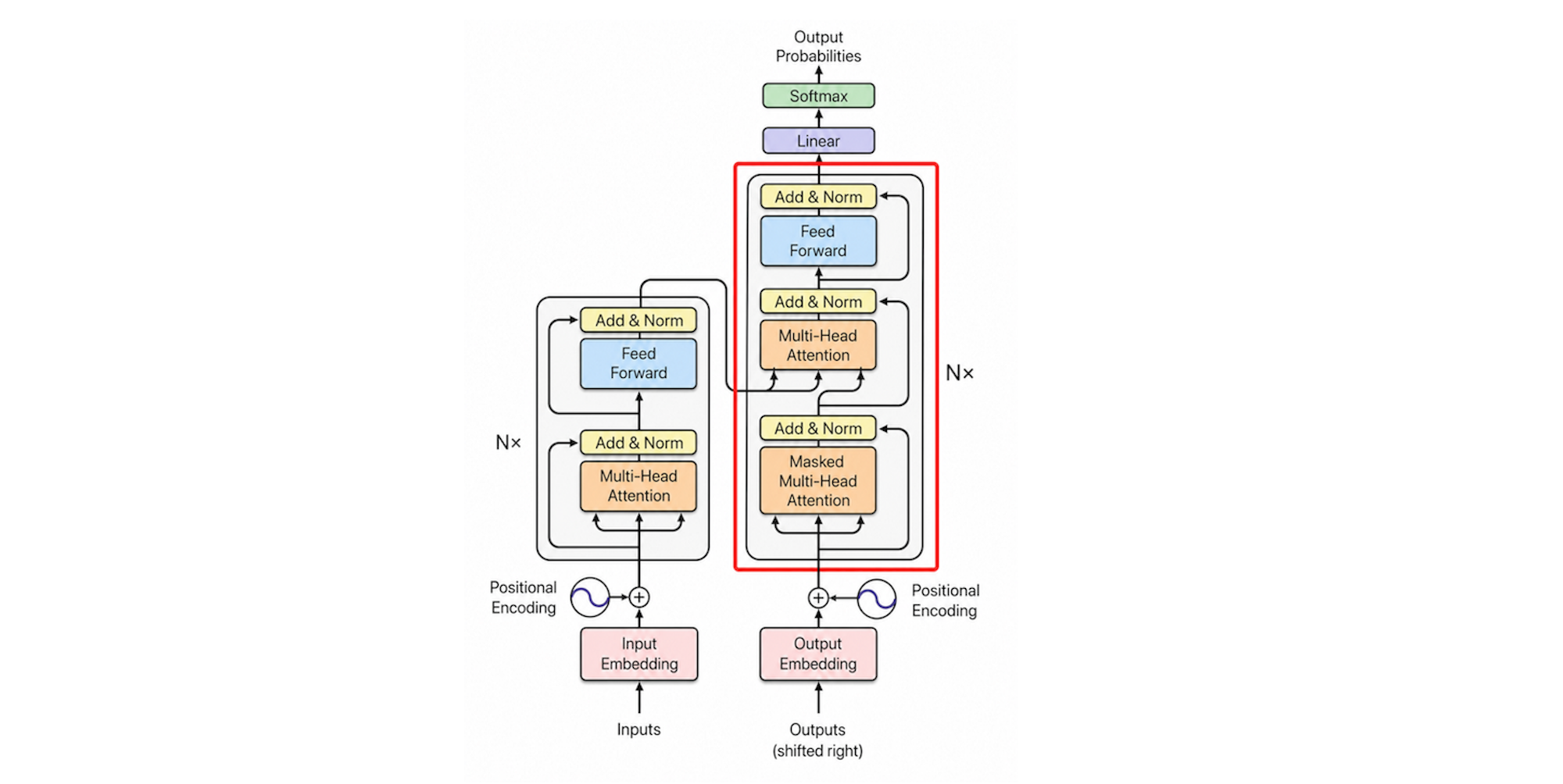
Everything here is general, public knowledge (see the Elastic overview linked at the end). There is no private or proprietary code involved. Because the original notes leaned heavily on diagrams, every figure below is redrawn as an ASCII flow so the post stays self-contained.
Glossary
The notation is dense, so here is the symbol table to read against:
- $d_{\text{model}}$: length of each token vector, and the total input/output width of multi-head attention (e.g. 512).
- $h$: number of attention heads.
- $d_k = d_v = d_{\text{model}} / h$: per-head dimension.
- $W_Q, W_K, W_V$: learned projection matrices producing Query / Key / Value.
- $W_O$: output projection applied after concatenating heads.
- $W_1, W_2$: the two weight matrices of the feed-forward network; the hidden width $d_{\text{ff}}$ is usually $4 \times d_{\text{model}}$.
- $W_{\text{out}}$: final projection to vocabulary logits, shape $d_{\text{model}} \times V$.
- $V$: vocabulary size (number of distinct token IDs).
- $X$: the input matrix (token embedding + positional embedding); one row per token.
- $Z$: attention block output; same shape as $X$.
The Big Picture
At the coarsest level, generating one token is three steps:
Step 1  Feature extraction
        token embedding  +  positional embedding  =  X

Step 2  Encoder / Decoder stack
        X  ->  [ attention + FFN, repeated N times ]  ->  Z

Step 3  Vocabulary projection
        Z  ->  x W_out  ->  logits over V tokens  ->  pick a token ID
Step 1 turns discrete tokens into vectors and injects word-order information (a bare bag of embeddings has no notion of position). Step 2 is where the model thinks: each token vector is repeatedly enriched with information about the other tokens it should attend to. Step 3 maps the final vector of each position onto the full vocabulary, producing a score for every possible next token.
A subtle but important point about Step 3: “pick the highest-scoring token ID” is only greedy decoding, one strategy among many. Real LLMs default to sampling by probability, which is exactly why the same prompt yields different outputs on different runs. More on that at the end.
Encoder
Encoder and Decoder blocks are nearly identical. Their shared building blocks are:
- Residual connection + layer normalization (Add & Norm)
- Multi-head attention
- Feed-forward network (FFN)
We’ll follow the Encoder’s execution order.
1. Linear projection into Q / K / V
The input $X$ (token embedding + positional embedding) is linearly projected by three matrices into Query, Key, and Value:
\[Q = X W_Q, \quad K = X W_K, \quad V = X W_V\]Each row of $Q$, $K$, $V$ corresponds to one token. In multi-head attention, $W_Q / W_K / W_V$ are sliced per head; each head computes attention independently, and the results are concatenated back together.
Assume $d_{\text{model}} = 512$, $h = 8$, so each head has $d_k = d_v = 512 / 8 = 64$. Conceptually:
- $Q$ is what the current token is asking about.
- $K$ is what each token can be matched against.
- $V$ is the information each token carries once matched.
For a single head, with sequence length 4, the shapes flow like:
\[\underbrace{X}_{4 \times d_{\text{model}}} \times \underbrace{W_Q}_{d_{\text{model}} \times d_k} = \underbrace{Q}_{4 \times d_k}\]The critical mental model: the $W$ matrices are fixed; Q/K/V are computed fresh from each input.
| Fixed? | Notes | |
|---|---|---|
| $W_Q, W_K, W_V$ | Yes | Learned during training, then frozen; identical for every input |
| $Q, K, V$ | No | Recomputed for each input; different $X$ gives different Q/K/V |
Think of $W_Q$ as a fixed “question machine”: the machine never changes, but feed it different words and it emits different query vectors. The attention table $S = \text{Softmax}(QK^\top / \sqrt{d_k})$ is likewise computed on the fly, never stored.
2. Scaled dot-product attention (per head)
With sequence length $L = 4$ and per-head dimension $d_k = 3$:
\[S = \text{Softmax}\!\left(\frac{Q K^\top}{\sqrt{d_k}}\right) V\]Reading it piece by piece:
- $Q K^\top$: $Q$ is $4 \times 3$, $K^\top$ is $3 \times 4$, so the product is $4 \times 4$. Entry $S_{ij}$ is the dot-product similarity between query $i$ and key $j$.
- Scaling by $\sqrt{d_k}$: prevents the dot products from growing so large that Softmax saturates (i.e. one entry dominating and gradients vanishing).
- Softmax: applied row by row, so each row sums to 1 — every token distributes a total attention weight of 1 across all tokens.
        k1   k2   k3   k4
     +---------------------+
 q1  | .7   .1   .1   .1   |  <- row sums to 1 after softmax
 q2  | .2   .6   .1   .1   |
 q3  | .1   .1   .5   .3   |
 q4  | .1   .2   .2   .5   |
     +---------------------+
       (S = attention weights, then multiplied by V)
3. Concatenate heads, then a linear projection
Each head independently produces an $L \times d_k$ output. Concatenate the $h$ heads side by side, then apply one output projection $W_O$. Using 8 tokens, $d_{\text{model}} = 512$, $h = 8$:
\[\text{Concat}(\text{head}_1, \dots, \text{head}_8) \in \mathbb{R}^{8 \times 512}\] \[\underbrace{\text{Concat}}_{8 \times 512} \times \underbrace{W_O}_{512 \times 512} = \underbrace{Z}_{8 \times 512}\]What is $Z$?
- Shape: $Z \in \mathbb{R}^{8 \times d_{\text{model}}}$ — exactly the same shape as the input $X$.
- Meaning: each row is still one token, but the vector now blends in that token’s attention over the rest of the sentence. Where $X$ held “isolated words,” $Z$ holds “words that have read the whole sentence and know what to focus on.”
- Why the shape must match $X$: the next step is a residual add, $X + Z$. For the addition to be valid the shapes must be identical, and $W_O$ projecting back to $d_{\text{model}}$ is precisely what guarantees it — while also letting the next Encoder layer continue at the same width.
   head_1  head_2   ...   head_8
   [8x64]  [8x64]         [8x64]
      \       |             /
       \      |            /
        concat  -> [8 x 512]
                       |
                    x W_O (512x512)
                       |
                    Z  [8 x 512]   (same shape as X)
4. Add & Norm
$Z$ then goes through Add & Norm — a residual add followed by layer normalization:
- Add (residual connection): computes $X + Z$, so the original token signal is never fully erased by attention. It also gives gradients a clean path back during training.
- Norm (layer normalization): keeps the feature values from drifting uniformly high or low and standardizes their spread, so no single dimension dominates.
LayerNorm operates per sample, across the feature dimension (not across the batch). For a single feature vector $x = [x_1, \dots, x_d]$ with $d = d_{\text{model}}$:
Step 1  mean      mu    = (1/d) * sum(x_i)
Step 2  variance  sigma = sqrt( (1/d) * sum((x_i - mu)^2) + eps )
Step 3  normalize x_hat_i = (x_i - mu) / sigma        -> mean 0, var 1
Step 4  scale/shift y_i   = gamma_i * x_hat_i + beta_i   (gamma, beta learned)
Step 5  output    y = [y_1, ..., y_d]  ->  next sub-layer
The learnable $\gamma$ and $\beta$ let the model undo part of the normalization when a layer actually needs a different scale. Placement varies: Pre-LN (normalize before the sub-layer) vs Post-LN (normalize after); modern models overwhelmingly favor Pre-LN for training stability.
5. Feed-forward network
After Add & Norm, each token vector passes through a small position-wise FFN — two linear layers with a nonlinearity between them:
\[\text{FFN}(x) = W_2 \, \phi(W_1 x + b_1) + b_2\]where $\phi$ is an activation such as ReLU / GELU / SwiGLU, and $d_{\text{ff}}$ (the hidden width) is typically $4 \times d_{\text{model}}$. Both $W_1$ and $W_2$ are learned by back-propagation. The FFN is applied independently to each position — it adds per-token nonlinear capacity, while attention is what mixes information across tokens.
A second Add & Norm follows the FFN. The whole block — attention, Add & Norm, FFN, Add & Norm — is then stacked $N$ times. The final layer’s $Z$ is what the Encoder hands off.
   X
   |
   v
 +-----------------------------+
 | Multi-Head Attention        |
 +-----------------------------+
   |                    ^
   +--> Add & Norm  <---+ (residual X)
   |
   v
 +-----------------------------+
 | Feed-Forward Network        |
 +-----------------------------+
   |                    ^
   +--> Add & Norm  <---+ (residual)
   |
   v
   Z   ---> repeat block N times
Decoder
A Decoder block mirrors the Encoder but contains two attention layers:
- Masked self-attention: Q, K, V all come from the Decoder’s own previous-layer output.
- Cross-attention: Q comes from this Decoder layer, while K and V come from the Encoder’s final output. This is how the decoder “consults” the encoded input.
Like the Encoder, the Decoder stacks its block $N$ times; the final output is passed on to the vocabulary projection.
Decoder-only models (Claude / GPT)
Everything above describes the original encoder-decoder Transformer. Modern mainstream models — Claude, GPT — are decoder-only, with a few key differences:
- No Encoder, no cross-attention. The “Q from decoder, K/V from encoder” cross-attention layer is removed entirely. Each layer has just one self-attention.
- Q / K / V all come from the input itself, exactly as in the Encoder’s step 1: $Q = X W_Q$, $K = X W_K$, $V = X W_V$. There is no “initial Q supplied by an encoder” — it comes straight from $X = \text{token emb} + \text{positional emb}$. Layer 1 derives Q/K/V from $X$; every later layer takes the previous layer’s output as its input:
- Causal mask. Self-attention is restricted so each token may only attend to itself and earlier tokens — never future ones, otherwise predicting the next token would be cheating. Concretely, in the $S = QK^\top$ matrix the “future” entries are set to $-\infty$, so after Softmax their weights become 0.
Causal mask on the attention scores S (rows = query, cols = key):

        k1   k2   k3   k4
   q1 [  x   -inf -inf -inf ]
   q2 [  x    x   -inf -inf ]
   q3 [  x    x    x   -inf ]
   q4 [  x    x    x    x   ]
        (-inf -> 0 after softmax: no peeking ahead)
| Original Decoder | Decoder-only (Claude / GPT) | |
|---|---|---|
| Has an Encoder | Yes | No |
| Cross-attention (Q from decoder, K/V from encoder) | Yes | No |
| Self-attention Q/K/V source | Input itself | Input itself |
| Initial $X$ | token emb + positional emb | token emb + positional emb |
| Causal mask | Yes | Yes |
Vocabulary Projection
Take $Z$ from the final Decoder layer:
\[Z_{\text{decoded}} \in \mathbb{R}^{d_{\text{tokens}} \times d_{\text{model}}}\]Apply the trained output projection:
\[W_{\text{out}} \in \mathbb{R}^{d_{\text{model}} \times V}\]The result is, for each position, a score across the entire vocabulary — the logits that become a probability distribution over next tokens:
\[H \in \mathbb{R}^{d_{\text{token}} \times V}\]$W_{\text{out}}$ is often weight-tied with the input embedding matrix, which saves parameters and tends to improve quality.
Why the Same Prompt Gives Different Answers
The entire forward pass — from $X$ all the way to the distribution $H$ — is deterministic, because at inference every weight ($W_Q, W_K, W_V, W_O, W_1, W_2, W_{\text{out}}$) is frozen. The randomness lives in one final step: which token to actually pick from $H$.
X -> (frozen-weight forward pass, deterministic) -> H -> [ sampling ] -> token
                                                            ^ randomness enters here
The knobs controlling that step are not part of the architecture — they are inference-time settings:
- temperature: scales logits ($z_i / T$) before Softmax. Higher $T$ flattens the distribution (more random); $T \to 0$ collapses to greedy (near-deterministic).
- top-k: sample only from the $k$ highest-probability tokens (fixed-size candidate set).
- top-p (nucleus): sample from the smallest set whose cumulative probability reaches $p$ (dynamic-size set).
- seed: fixing the RNG seed plus all other settings makes runs reproducible.
As long as temperature > 0, the last step is not “take the max” but “roll the dice by probability,” so the second-ranked token can win — and outputs vary. To pin output down: temperature = 0 (or near-zero) plus a fixed seed.
One counter-intuitive caveat: even at temperature = 0, large models are not always bit-for-bit reproducible. GPU floating-point addition is not associative — parallel reduction order and the mix of other requests in the same batch cause tiny logit jitter. Usually harmless, but when the top-two scores are extremely close it can flip the argmax, and autoregression amplifies the divergence token by token. This is why production APIs offering a seed promise only best-effort reproducibility.
Wrap
Read top to bottom, the Transformer is a short list of repeated moves: project into Q/K/V, score with scaled dot-product attention, mix per head and project back, stabilize with Add & Norm, add per-token nonlinearity with the FFN, stack $N$ times, then map to the vocabulary. The two things worth internalizing are (1) the weights are frozen while Q/K/V are recomputed from every input, and (2) the attention output deliberately keeps the input’s shape so residuals compose and layers stack cleanly. Modern decoder-only models drop the encoder and cross-attention, keep a single causal self-attention per layer, and push all the remaining variety in behavior into the sampling step at the very end.
Background reference: What is a large language model? (Elastic)